User's Guide

What's In A Line? is a Java applet designed to help teach four computer graphic scan conversion algorithms. This guide is intended to help web surfers get started and use the What's In A Line? applet. It contains a section on getting started and subsequent sections describing the operation of all parts of the program. There are also sections that describe how the scan conversion algorithms work.

A Quick Start:

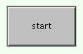
To launch the applet, simply click on the big Start button at the top of the project page. The button looks like this:

When a Java applet is launched, Java code is downloaded from the server to your browser. Sometimes this download can take a long time. Only click on the Start button once. If you press it more than once you will end up with more than one instance of the program. If the applet window does not appear after a minute, check your browser's Java console for errors.

The line drawing applet consists of just one window. Everything you need to use the program is right there in front of you. The pink area in the upper right-hand corner is the Drawing Area. That's where you define the lines and circles that you'll be rendering. To get started, move your mouse cursor into the pink area. Press and hold the button on your mouse . Drag the mouse a short distance. Release the mouse button. You have just defined a line that will be rendered by the Midpoint Line Algorithm.

Down in the lower left-hand corner of the window you'll see several square buttons. Click the Run button. You'll notice that the line in the Drawing Area gets rendered in black - the Midpoint Line Algorithm was applied to the line you defined with your mouse. You will also notice that the purple area in the lower right-hand corner also had some activity in it. The purple area is the Zoom Panel. The Zoom Panel is a "close-up" view into the Drawing Area.

Now you know the basics of using the What's In A Line? applet. Experiment with different lines in the Drawing Area. The rest of this document describes the full functionality of the applet. It tells you how to change algorithms, monitor execution, set breakpoints and view the rendered primitives in detail. Good luck!

Changing Algorithms:

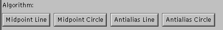
What's In A Line? comes with four algorithms that you can investigate; Midpoint Line Algorithm, Midpoint Circle Algorithm, Antialiased Midpoint Line Algorithm and Antialiased Circle Algorithm. The first three algorithms are taken directly from Computer Graphics: Principles and Practice, by Foley, vanDam, Feiner and Hughes. The Antialiased Circle Algorithm is an adaptation of the Midpoint Circle Algorithm and general antialiasing principles. Foley has excellent sections on theory and practice for antialiasing. A more brief explanation of each algorithm is given later in this manual.

The four buttons in the upper left-hand corner of the applet let you select the algorithm of your choice.

When the applet is first launched, the Midpoint Line Algorithm is displayed in the Code Window by default. You will notice that as you choose between the algorithms the code in the Code Window changes. The Code Window has scrollbars attached to it so you can review the source as you wish.

If you have already drawn a primitive in the Drawing Area you will notice that changing algorithms also changes the primitive in the Drawing Area.

Switching between algorithms resets any drawing in the Drawing Area and clears any parameters for the current algorithm. In other words, if you are halfway through an algorithm and switch to another one, the data in the first algorithm is erased.

Defining Primitives:

The pink area in the upper right-hand corner of the applet is the main Drawing Area. Your mouse is used to interactively define two points for rendering primitives. Pressing the mouse button defines the first point (P1) and releasing the mouse button defines the second point (P2). Dragging the mouse animates a primitive using the first point (P1) and the cursor position. You can "pick-up" and move an existing point by placing your cursor over the point and pressing the mouse button.

Both lines and circles are defined by P1 and P2 . The primitive you see depends on which algorithm is currently selected. When a line algorithm is currently selected, P1 and P2 represent the endpoints of a line. For the circle algorithms, P1 and P2 represent the radius of a circle where P1 is at the center and P2 is on the circumference of the circle.

Note: P1, P2 and the primitives they define are clamped to the boundaries of the pink canvas. When P1 and P2 are defined in line mode and are near the edge of the Drawing Area it may not be possible to convert P1 and P2 to a corresponding circle without drawing part of it off the edge of the canvas. In this case, the endpoints are automatically repositioned so the entire circle will be visible in the drawing area. The original points are not preserved when this clamping occurs.

P1 and P2 can also be modified from the Feedback Panel. Click on one of the endpoint parameter text fields and enter a numeric value. The new value does not take effect until you press the "Enter" key. When all four fields are filled in, the Drawing Area will be updated accordingly.

Controlling Rendering:

The six square buttons in the lower left-hand corner of the applet control rendering.

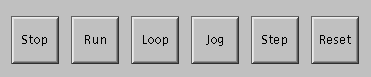
The Stop button halts execution of an algorithm that is currently rendering.

The Run button executes the algorithm at full speed and draws the line or circle in the Drawing Area. For performance reasons the Zoom Panel is only updated periodically and lines of code in the Code Window are not highlighted interactively.

The Loop button is intended to work in conjunction with a breakpoint. See Setting A Breakpoint for information on how to do that. The Loop button executes the current algorithm at full speed, rendering each pixel to the Drawing Area and Zoom Panel. It also highlights each line of code in the Code Window. By setting the breakpoint and using the Loop button, you can stop at the same point every time through the main loop of an algorithm allowing you to examine specific variables, the Drawing Area and the Zoom Panel.

The Jog button executes the algorithm slowly - approximately 1 statement per second. Jog provides a slow motion animation as the applet steps through the algorithm and renders the primitive one pixel at a time.

The Step button advances the algorithm one statement each time it is pressed. it is ideal for reviewing the changes to critical algorithm variables at each line of code. It allows you to proceed at your own pace and see how an algorithm works step by step.

The Reset button clears the Drawing Area and Zoom Panel of any rendered pixels, resets the algorithm, and resets all algorithm variables.

All six buttons work in conjunction with each other. For instance, if the algorithm is currently jogging and you press the Run button, execution will complete at full speed. Or, you could Jog the algorithm until you hit your breakpoint for the first time and continue with the Loop button.

The Feedback Panel:

Just above the control buttons and below the Code Window is the Feedback Panel. It contains a small status text area, the breakpoint controls, and a collection of variables associated with the current algorithm. The control panel for the Midpoint Line Algorithm looks like this:

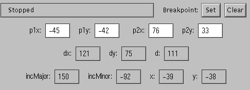
The status area displays the "state" of the algorithm. The state is either: "Stopped", "Running", "Looping", "Jogging", "Stepping", or "Resetting". When you Set, Clear or Stop at a breakpoint, there is a brief confirmation message displayed in the Status window.

Setting a Breakpoint is discussed in the next section.

The remaining labels and text fields represent the various parameters and variables of the current algorithm. You will notice that the fields change from algorithm to algorithm. The labels that appear to the left of the values correspond to variables in the algorithm. Not all algorithm variables are represented in the Feedback Panel - just the ones that are important to rendering the primitive.

You are allowed to edit the fields for P1 and P2 (editable fields are highlighted in white). For the line algorithms, P1 and P2 are the endpoints of the line. For the circle algorithms, P1 and P2 define the radius of a circle with P1 at the center and P2 on the circumference of the circle. The ability to edit the line endpoints is important because setting exact endpoints with your mouse can be difficult . See Defining Primitives for more information.

Setting A Breakpoint:

What's In A Line? allows you to set one breakpoint in the Code Window. All of the automatic rendering modes (Run, Loop, Jog) will stop at the breakpoint. The breakpoint is handy if you want to see if certain parameters result in the execution of a certain portion of code or if you want to check the values of some variables each time thru the main loop of an algorithm.

To set a breakpoint, first highlight a single line of text in the Code Window. The line must be highlighted completely from left to right. If more or less than one complete line of code is highlighted, the breakpoint cannot be set. This restriction has its roots in the Java implementation of the text window.

The easiest way to highlight a single line of code is to triple-click on it. The mouse can be used to drag it, but this is more difficult.

Press the Set button in the Feedback Panel. The status area will tell you if setting the breakpoint was successful.

To clear a breakpoint simply press the Clear button.

Remember there is only one breakpoint. If it is set more than once, only the most recent breakpoint will be in effect.

The Zoom Panel:

The Zoom Panel is the purple panel that appears in the lower right portion of the applet. Its function is to be a "magnifying glass" into the Drawing Area. Pixels in the Zoom Panel are between 10 and 50 times as large as those in the Drawing Area. You can control the magnification with the little pull-down menu that lives between the Control Panel and the Zoom Panel.

During rendering of a primitive, the Zoom Panel will follow the drawing of pixels - any time a pixel is rendered out of view, the Zoom Panel will re-center itself so the current set of pixels are always visible. Scrollbars are provided if you wish to navigate a rendered primitive at any time.

The Midpoint Line Algorithm:

Before launching into an explanation of the midpoint line algorithm, it's important to consider the properties that make up a "good" line. First of all, a line, in the theoretical sense, is an infinitely thin, straight connection between two infinitely small points. But a computer screen consists of thousands or millions of pixels with a specific size. Representing a line with a collection of fixed size pixels is an approximation.

To achieve the best approximation possible, we should choose the pixels that lie as close to the true line as possible. The collection of pixels should also appear straight, that is, it should be accurate. Consistent brightness is also important. And since the theoretical line is thin, the rendered line should be thin as well - preferably one pixel thick. Of course there are cases where thick lines are desired, but they are out of the scope of this project. To achieve these goals we would like to illuminate one pixel per column in a uniform manner for all lines with slope -1 to 1 and one pixel per row for all other slopes. Finally, any line algorithm should be very fast since it is likely to be a heavily used part of any graphics system.

In the field of computer graphics the discussion often arises as to whether the coordinate of a pixel lies at its center or one of its corners. Rather than debate this issue here, it is assumed that the coordinate of the pixel is at its center. This assumption is clearly visible in the Zoom Panel of the What's In A Line? applet.

The following description of the midpoint line algorithm applies to all lines with slope between 0 and 1. All other slopes can be handled by modifying the algorithm to reflect the line about the major or minor (y = x, y = -x) axes. In all, there are eight cases to be considered: [0,1], (1, oo], (0, -1], (-1, oo] where P1x <= P2x, and [0,1], (1, oo], (0, -1], (-1, oo] where P1x > P2x. What's In A Line? works for all these cases. However, code is provided for some of them while pseudo-code is provided for the remainder. As an exercise, try deriving the code for the remaining slope cases yourself.

The midpoint line algorithm is widely used because it meets all the criteria of a good line algorithm; it has been proven to choose the pixels closest to the line (accuracy, consistency, straightness), it chooses only one pixel per column, and it is very fast. Its speed and compactness are probably why it is so popular. The midpoint line algorithm uses only integer arithmetic and does no multiplication or division in its main loop.

The basis for the midpoint line algorithm is simple. Given the previous pixel selection P, there are two candidates for the next pixel closest to the line, E and NE (E stands for East and NE stands for Northeast). M is the midpoint between them. Decide on which side of M the line passes and choose the pixel which is closest to the line. If the M is above the line, choose E. If M is below the line, choose NE. This is obvious from the drawing below (The drawing is from Foley, p. 76. The grid lines are at pixel centers. The empty circles are background pixels. The black circle is a shaded pixel):

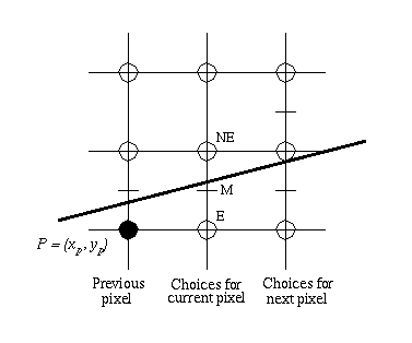
The midpoint line algorithm visits every column of pixels from the start point to the end point. Since the start point is on the line, it serves as the first "previous" pixel to prime the algorithm.

The implicit equation of a line is:

F(x, y) = ax + by + c

For all points on the line, the solution to F(x, y) is 0. All points above F(x, y) result in a negative number and all points below F(x, y) result in a positive number. This relationship is used to determine the relative position of M.

The decision variable, d, is derived from the implicit form of a line. The sign of d is used to make the midpoint determination for all remaining pixels. If d is positive, the midpoint is below the line and NE is chosen. If d is negative or zero, the midpoint is above the line and E is chosen. As the algorithm progresses from pixel to pixel, d is incremented with one of two precalculated values based on the E/NE decision. When using the line algorithm with lines of moderate slope, pay special attention at how the value of d oscillates back and forth between positive and negative.

For the complete mathematical derivation of the midpoint line algorithm, see Foley, pp. 76- 77.

The Midpoint Circle Algorithm:

A circle has symmetric properties that can be exploited when rendering on a raster display. For circles centered at the origin, the four quadrants are mirror images of each other. However, if a single quadrant of a circle is scan converted in one dimension, pixel continuity goes away as the slope passes +/- 1. If the circle is divided into eights and pixels are mirrored about y = x and y = -x as well as the major axes, pixel continuity is maintained.

The midpoint circle algorithm takes advantage of eight way symmetry by calculating just the pixels in the second octant (slope = [1, oo]) and mirroring into all the others. Circles that are not centered at the origin can be re-oriented with a simple translation.

The strategy of the midpoint circle algorithm is the same as the midpoint line algorithm; given the last pixel, decide which pixel to visit next based on where the theoretical arc of the circle passes with respect to the midpoint between the two prospective pixels. Here's a drawing from Foley, p. 83:

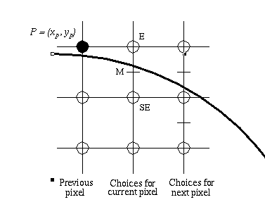
Scan conversion starts at x = 0 and visits each column in the positive x direction as long as the resulting y values continue to be greater than or equal to the current x value. When y <= x, all the pixels in the quadrant have been rendered.

The implicit function of a circle is:

F(x, y) = x² + y² + R

F(x, y) is 0 for all (x, y) on the circle. The result is positive for all points outside the circle and negative for all points inside the circle. This relationship is used to determine the relative location of M with respect the theoretical circle.

The decision variable, d, is derived from the implicit form of a circle. At each pixel, d is used to choose between the E (East) and SE (Southeast) pixel. As with the midpoint line algorithm, the sign of d indicates whether the midpoint is inside (below) or outside (above) the circle. If d is positive or zero, the midpoint is outside the circle and SE is chosen. If d is negative, the midpoint is inside the circle and E is chosen. As the algorithm progresses from pixel to pixel, d is incremented based on the E/SE decision. In contrast to the line algorithm where the incremental values are precalculated, the values used to increment d in the circle algorithm are constantly changing. This is because the slope of the circumference is constantly changing. The incremental value of d is based on the new values of x and y.

For a complete mathematical derivation of the midpoint circle algorithm, see Foley, pp.83 - 85.

Special Note: The midpoint circle algorithm uses only integer arithmetic and only works for circles who's center is at the origin and radius is an integer value. Applying a simple translation transformation eliminates the center-at-origin restriction. However, the technique used to define circle primitives in the the Drawing Area can give rise to circles with non-integer radii. What's In A Line? rounds any non-integer radius before applying the circle algorithm. When rounding is significant, some of the pixels rendered in the Zoom Panel appear to be incorrect. To minimize the roundoff error, try to keep the radius of the circle in the Drawing Area completely horizontal or vertical. Roundoff error is introduced when the slope of the radius deviates from 0 or oo.

The Antialiased Line Algorithm:

When you look at lines rendered by the midpoint line algorithm in the Zoom Panel you will notice that they are very rough. They have a significant "staircase" effect that is commonly called "the jaggies". Roughness or the jaggies are more accurately called aliasing. Aliasing is a result of choosing the pixel nearest to an infinitely thin line and coloring it full-on with a foreground color such as black. Antialiasing is the application of techniques to reduce or eliminate aliasing. Aliasing and antialiasing are related to signal and sampling theory. A theoretical discussion of either of these topics is outside the scope of this project. An informal description of an antialiasing technique applied to the midpoint line algorithm follows.

The antialiased line algorithm is based on the midpoint line algorithm. The same decision variable, d, and sequence are used to decide which pixel is closest to the line. Once that pixel is determined, the distance from the pixel's center to the line is calculated. Further, the distance from its two vertical neighbors to the line is also calculated. These distances are normalized and used as factors for picking each corresponding pixel's intensity - an intensity that is proportional to the pixel's distance from the line. In other words, the closer a pixel is to the line, the darker it is. The farther away a pixel is from the line, the lighter it is.

Calculating the distance between a pixel center and a line is costly and time consuming. It involves floating point numbers, multiplication, division and a square root calculation. To minimize this calculation, the antialias line algorithm takes advantage of the incremental calculation of d and the fact that the slope of the line is constant. Because of this, much of the distance formula can be precomputed and some of the mathematical overhead is eliminated. The derivation of the incremental distance calculation is not difficult, but it is a little lengthly. See Foley, p. 137 - 140 for the complete derivation.

The Antialiased Circle Algorithm:

The antialiased circle algorithm is very similar to the midpoint circle algorithm. The decision variable, d, is used to select the pixels that lie closest to the arc in the second octant. As each pixel is chosen, the antialiasing technique is applied. The distance between the center of the current pixel and the line is calculated, normalized, and used as a factor for calculating the intensity of the pixel. For each of the pixel's vertical neighbors (one above and one below) the same distance calculation is applied to generate an intensity value.

The antialiased circle algorithm trades speed for complexity. Where the antialiased line algorithm used the incremental nature of d to minimize mathematical calculation, the antialiased circle algorithm performs a brute force distance calculation for every pixel. Overall the algorithm is slower, but its appearance is much cleaner and there are fewer variables in the code.